Did you know that you can navigate the posts by swiping left and right?

인공지능 프로젝트

09 Jun 2020 . category: tech . Comments
#mechatronics #AI #hunkim #pytorch

수업 인공지능을 배우고 이를 이용하여 실제로 적용하는 프로젝트를 진행하였다.

작품의 목표로는 주행하는 자동차가 표지판을 인식하여 속도 조절 및 멈추는 것을 목표로 하였다. 3가지로 classification 후 주행을 통해 속도 조절로 이를 구형하였다. 우선 그래픽 카드가 장착된 컴퓨터에서 학습을 진행한 후 학습된 데이터를 jetsonnano로 가져와 자동차와 연동하여 구동하도록 프로젝트를 진행하였다.

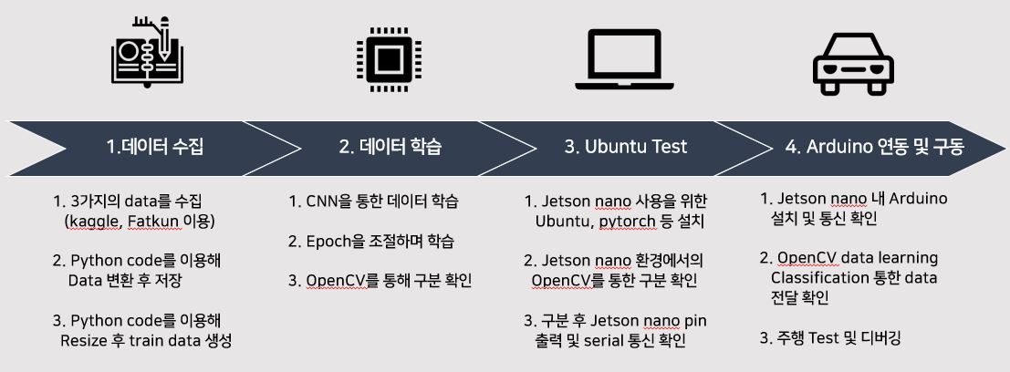
데이터는 kaggle과 구글 페이지의 이미지 검색을 통해 얻을 수 있고 이를 통해 총 3가지의 data 수집을 하였다. 각 1000개 씩의 train_data와 100개의 test data를 구성하였고 총 3300개의 데이터를 학습에 이용하였다.

학습을 하기 전에 각각의 데이터에 라벨을 지정하기 위해 코드를 구성하였는데 각 이미지에 라벨을 지정해 따로 저장하는 python 코드는 다음과 같다.

import torchvision
from torchvision import transforms

from torch.utils.data import DataLoader
from matplotlib.pyplot import imshow

from PIL import ImageFile
ImageFile.LOAD_TRUNCATED_IMAGES = True

trans = transforms.Compose([transforms.Resize((256,256))])

train_data = torchvision.datasets.ImageFolder(root='custom_data/origin_data', transform=trans)
for num, value in enumerate(train_data):
    data, label = value
    print(num, data, label)
    
    if(label == 0):
        data.save('custom_data/train_data/car_go/%d_%d.jpeg'%(num,label))
    if(label == 1):
        data.save('custom_data/train_data/child/%d_%d.jpeg'%(num,label))
    if(label == 2):
        data.save('custom_data/train_data/stop/%d_%d.jpeg'%(num,label))

위 코드는 torch와 torchvision에서 제공하는 기본 코드를 이용한 코드이다.

import torch
import torch.nn as nn
import torch.nn.functional as F

import torch.optim as optim
from torch.utils.data import DataLoader

import torchvision
import torchvision.transforms as transforms

import matplotlib.pyplot as plt

import cv2
import numpy as np
import sys

device = 'cuda' if torch.cuda.is_available() else 'cpu'
    
trans = transforms.Compose(
    [transforms.Resize([256,256]),
     transforms.ToTensor(),   
     transforms.Normalize((0.5, 0.5, 0.5), (0.5, 0.5, 0.5))])

train_data = torchvision.datasets.ImageFolder(root='./custom_data/origin_data', transform=trans)
train_loader = torch.utils.data.DataLoader(train_data, batch_size=4, shuffle=True)

count = 1
file_name_path = './custom_data/origin_data/car_go/image'+str(count)+'.jpg'
file_name_path2 = './custom_data/img_change3/image'+str(count)+'.jpg'

def transform():
    file_name_path = './custom_data/origin_data/car_go/image'+str(count)+'.jpg'
    file_name_path2 = './custom_data/img_change3/image'+str(count)+'.jpg'
    img = cv2.imread(file_name_path)
    h, w = img.shape[:2]
    M1 = cv2.getRotationMatrix2D((w/2, h/2), -30, 1)
    img2 = cv2.warpAffine(img, M1, (w, h))
    img_gray = cv2.cvtColor(img, cv2.COLOR_BGR2GRAY) 
    #cv2.imwrite(file_name_path2, img2)
    cv2.imwrite(file_name_path2, img_gray)
    cv2.waitKey(0)
    cv2.destroyAllWindows()
    
    
while True:
    transform()
    count+=1 
    if count == 514:
        break
print('Colleting Samples Complete!!!')

Origin data를 변형하여 데이터의 개수를 늘려 주었다. 이 이유는 저장한 데이터를 색깔로만 구별할 수도 있고 이미지가 기울어지거나 명도에 따라 달라질 수 도 있기에 각도 변형한 데이터, 그레이 스케일 이미지를 따로 만들어 저장하였다. 각 3개의 데이터를 일일이 적용해 변형하여 저장하였다.

import torch
import torch.nn as nn
import torch.nn.functional as F

import torch.optim as optim
from torch.utils.data import DataLoader

import torchvision
import torchvision.transforms as transforms
from torchvision import datasets, transforms
from torch.utils.data import DataLoader

import matplotlib.pyplot as plt

import cv2
import numpy as np
import sys

device = 'cuda' if torch.cuda.is_available() else 'cpu'

    
trans = transforms.Compose(
    [transforms.Resize([256,256]),
     transforms.ToTensor(),   
     transforms.Normalize((0.5, 0.5, 0.5), (0.5, 0.5, 0.5))])

train_data = torchvision.datasets.ImageFolder(root='./custom_data/train_data', transform=trans)
#data_loader = DataLoader(dataset = train_data, batch_size = 8, shuffle = True, num_workers=2)
train_loader = torch.utils.data.DataLoader(train_data, batch_size=8, shuffle=True)

classes = ('car_go','child','stop')
testLoss = []
trainLoss = []

def letterbox_image(img, inp_dim):
    '''resize image with unchanged aspect ratio using padding'''
    img_w, img_h = img.shape[1], img.shape[0]
    w, h = inp_dim
    new_w = int(img_w * min(w/img_w, h/img_h))
    new_h = int(img_h * min(w/img_w, h/img_h))
    resized_image = cv2.resize(img, (new_w,new_h), interpolation = cv2.INTER_CUBIC)
    
    canvas = np.full((inp_dim[1], inp_dim[0], 3), 128)

    canvas[(h-new_h)//2:(h-new_h)//2 + new_h,(w-new_w)//2:(w-new_w)//2 + new_w,  :] = resized_image
    
    return canvas

def pre_image(imgs):
    orig_im = imgs
    dim = orig_im.shape[1], orig_im.shape[0]
    imgs = (letterbox_image(orig_im, (256,256)))
    imgs_ = imgs[:,:,::-1].transpose((2,0,1)).copy()
    imgs_ = torch.from_numpy(imgs_).float().div(255.0).unsqueeze(0)
    return imgs_,orig_im, dim
    

class CNN(nn.Module):
    def __init__(self):
        super(CNN, self).__init__()
        self.layer1 = nn.Sequential(
            nn.Conv2d(in_channels=3, out_channels=6, kernel_size=5), #(in_channels=3, out_channels=6, kernel_size=5, padding=2
            nn.ReLU(),
            nn.MaxPool2d(2),
        )
        self.layer2 = nn.Sequential(
            nn.Conv2d(in_channels=6, out_channels=16, kernel_size=5),
            nn.ReLU(),
            nn.MaxPool2d(2),
        )
        self.layer3 = nn.Sequential(
            nn.Linear(16*61*61, 120), #16=Conv2d의 출력 채널, 13*29= image dimension
            nn.ReLU(),
            nn.Linear(120,84),
            nn.Linear(84,3)
        )
        
    def forward(self, x):
        out = self.layer1(x)
        out = self.layer2(out)
        out = out.view(out.size(0), -1)
        out = self.layer3(out)
        return out
    
net = CNN().to(device)

optimizer = optim.SGD(net.parameters(), lr=0.0001, momentum=0.9)
loss_func = nn.CrossEntropyLoss().to(device)

total_batch = len(train_loader)
net.train()
epochs = 25
for epoch in range(epochs):
    avg_cost = 0.0
    running_loss = 0.0
    for num, data in enumerate(train_loader):
        imgs, labels = data
        imgs = imgs.to(device)
        labels = labels.to(device)
        optimizer.zero_grad()
        out = net(imgs)
        loss = loss_func(out, labels)
        loss.backward()
        optimizer.step()
        
        running_loss +=loss.item()
        avg_cost += loss / total_batch
        
    print('[Epoch:{}] cost = {}'.format(epoch+1, avg_cost))
    trainLoss.append(running_loss / len(train_loader))
print('Learning Finished!')

torch.save(net.state_dict(), "./model/model.pth")
new_net = CNN().to(device)
new_net.load_state_dict(torch.load('./model/model.pth'))

print(net.layer1[0])
print(new_net.layer1[0])

print(net.layer1[0].weight[0][0][0])
print(new_net.layer1[0].weight[0][0][0])
net.layer1[0].weight[0] == new_net.layer1[0].weight[0]

trans= torchvision.transforms.Compose([transforms.Resize((256,256)), transforms.ToTensor()])
test_data = torchvision.datasets.ImageFolder(root='./custom_data/test_data', transform=trans)

test_set = torch.utils.data.DataLoader(dataset=test_data, batch_size=len(test_data), shuffle=True)
epochs = 5
for epoch in range(epochs):    
    with torch.no_grad():
        testing_loss = 0.0
        for num, data in enumerate(test_set):
            imgs, labels = data[0].to(device), data[1].to(device)
            prediction = new_net(imgs)
            loss = loss_func(prediction,labels)
            testing_loss +=loss.item()
            correct_prediction = torch.argmax(prediction, 1) == labels
            accuracy = correct_prediction.float().mean()
            print('Accuracy:', accuracy.item())
        testLoss.append(testing_loss /len(test_set))

# Loss graph
plt.figure(0) 
plt.title('Learning curve')      
plt.plot(trainLoss,label='Train loss')
plt.legend()

plt.figure(1)
plt.title('learning curve')
plt.plot(testLoss,label='test loss')
plt.legend()

데이터 학습을 위해 전처리 선언

transfoms.Compose를 통해 이미지를 resize로 똑같은 크기로 설정해주고 ToTensor를 통해 0~1사이의 값으로 변경 다시 Normalize를 통해 -1~1사이의 값으로 변경한다. train_data 폴더의 데이터들을 위 변경 선언들을 적용해 가져오고 batch_size = 8단위로 뽑아 가져오게된다.

class는 car_go, child, stop으로 3개를 선언해준다.

학습을 위한 CNN 선언

nn.Conv2d를 통해 Convolution을 수행하고 nn.MaxPool2d를 통해 pooling 수행한다. nn.Linear와 nn.ReLU 활성화 함수를 통해 최종적으로 3개의 output이 출력된다.

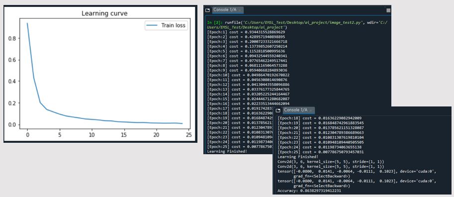
Train_data 기반 학습

optim.SGD를 통해 gradient decent를 적용하고 nn.CrossEntropyLoss를 통해 loss를 취득한다. avg_cost 변수에 손실값을 저장해 epoch 한번당 cost를 확률로 보게 된다. 예측값과 라벨값을 loss_func을 거쳐 loss변수에 저장하고 torch.argmax를 통해 해당되는 라벨값을 추적하게 된다. 평균으로 나누어 맞춘 정확도(accuracy)를 출력한다.

학습 후 jetsonnano를 통한 실시간 구동

최종 목표인 jesonnano 구동을 위해 우선 Ubuntu 18.0.4 환경을 이용하였다. 인공지능을 통해 구분 역할에 torch,torchvision을 설치하고 실시간 비전 시스템인 opencv 프로그램을 이용하였다. 앞서 말했듯이 window 환경 컴퓨터에서 학습된 model.pth을 가져와 OpenCV의 Classification을 진행하였다.

import torch
import torch.nn as nn
import torch.nn.functional as F

import torch.optim as optim
from torch.utils.data import DataLoader

import torchvision
import torchvision.transforms as transforms
from torchvision import datasets, transforms
from torch.utils.data import DataLoader

import matplotlib.pyplot as plt

import cv2
import numpy as np
import sys

device = 'cuda' if torch.cuda.is_available() else 'cpu'

trans = transforms.Compose(
    [transforms.Resize([256,256]),
     transforms.ToTensor(),   
     transforms.Normalize((0.5, 0.5, 0.5), (0.5, 0.5, 0.5))])

def letterbox_image(img, inp_dim):
    '''resize image with unchanged aspect ratio using padding'''
    img_w, img_h = img.shape[1], img.shape[0]
    w, h = inp_dim
    new_w = int(img_w * min(w/img_w, h/img_h))
    new_h = int(img_h * min(w/img_w, h/img_h))
    resized_image = cv2.resize(img, (new_w,new_h), interpolation = cv2.INTER_CUBIC)
    
    canvas = np.full((inp_dim[1], inp_dim[0], 3), 128)

    canvas[(h-new_h)//2:(h-new_h)//2 + new_h,(w-new_w)//2:(w-new_w)//2 + new_w,  :] = resized_image
    
    return canvas

def pre_image(imgs):
    orig_im = imgs
    dim = orig_im.shape[1], orig_im.shape[0]
    imgs = (letterbox_image(orig_im, (256,256)))
    imgs_ = imgs[:,:,::-1].transpose((2,0,1)).copy()
    imgs_ = torch.from_numpy(imgs_).float().div(255.0).unsqueeze(0)
    return imgs_,orig_im, dim
    

class CNN(nn.Module):
    def __init__(self):
        super(CNN, self).__init__()
        self.layer1 = nn.Sequential(
            nn.Conv2d(in_channels=3, out_channels=6, kernel_size=5), #(in_channels=3, out_channels=6, kernel_size=5, padding=2
            nn.ReLU(),
            nn.MaxPool2d(2),
        )
        self.layer2 = nn.Sequential(
            nn.Conv2d(in_channels=6, out_channels=16, kernel_size=5),
            nn.ReLU(),
            nn.MaxPool2d(2),
        )
        self.layer3 = nn.Sequential(
            nn.Linear(16*61*61, 120), #16=Conv2d의 출력 채널, 13*29= image dimension
            nn.ReLU(),
            nn.Linear(120,84),
            nn.Linear(84,3)
        )
        
    def forward(self, x):
        out = self.layer1(x)
        out = self.layer2(out)
        out = out.view(out.size(0), -1)
        out = self.layer3(out)
        return out
    
net = CNN().to(device)

optimizer = optim.SGD(net.parameters(), lr=0.0001, momentum=0.9)
loss_func = nn.CrossEntropyLoss().to(device)

new_net = CNN().to(device)
new_net.load_state_dict(torch.load('./model/model.pth'))

trans= torchvision.transforms.Compose([transforms.Resize((256,256)), transforms.ToTensor()])
cap = cv2.VideoCapture(0) # video 캡쳐 객체 생성

info = ''
cnt = 0
while(True):
    ret, img_color = cap.read()
    if ret == False:
        continue
    imgs, orig_im, dim = pre_image(img_color)
    imgs = imgs.cuda()
    
    new_net = CNN().to(device)
    new_net.load_state_dict(torch.load('./model/model.pth'))
    prediction = new_net(imgs)
    cv2.imshow('Color',img_color)
    if cv2.waitKey(1)&0xFF == 27:
        break
    detect = torch.argmax(prediction, 1)
    cnt = cnt+1
    if cnt >30:
        if(detect == 0):
            print("car_go is here")
            print("camera1 : {}".format(torch.argmax(prediction, 1)))
            cnt = 0
        if(detect == 1):
            print("child is here!")
            print("camera1 : {}".format(torch.argmax(prediction, 1)))
            cnt = 0
        if(detect == 2):
            print("stop is here!")
            print("camera1 : {}".format(torch.argmax(prediction, 1)))
            cnt = 0
cap.release()
cv2.destroyAllWindows()

jesonnano를 통해 classification을 수행

cv2.VideoCaputre를 통해 객체를 생성하고 cap read를 통해 비디오를 읽어들인다. pre_image를 통해 OpenCV 이미지를 네트워크 입력으로 사용하도록 변형한다. cv2.imshow로 실시간 비디오 확인하면서 구동을 확인한다.

cnt 기반 값마다 현재 인지된 상황을 분류하게 되고 detect = 0 (car_go - 주행 표지판) detect = 1 (child - 어린이 표지판) detect = 2 (stop - 정지 표지판)

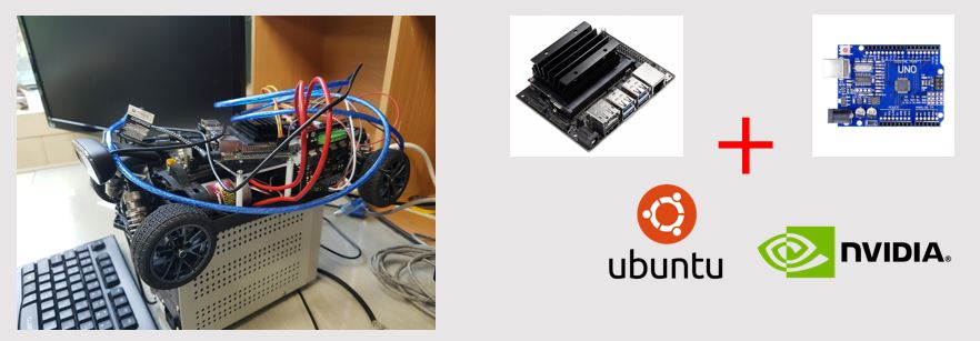
하드웨어는 다음과 같이 구성하였고

위 영상으로 최종 구동을 확인하였다.

github를 이용해 만들어본 블로그입니다.